Susceptible depletion in the renewal model

Epinowcast Team

The renewal expectation model in epinowcast can optionally account for susceptible depletion. Given an initial susceptible population, transmission is scaled by the remaining susceptible fraction, so the effective reproduction number bends down as the pool depletes. This vignette demonstrates the adjustment on simulated data where depletion plays a clear role, fitting the expectation-only model with and without it.

Code

library(epinowcast)
library(data.table)
library(ggplot2)

set.seed(2024)

A depleting epidemic on simulated data

We simulate a single well-mixed population of N = 4000 susceptibles seeded with a few cases and driven by a renewal process with a fixed generation time and a constant reproduction number. Because the population is small, the susceptible pool is depleted over the epidemic, so the wave peaks and then declines even though transmissibility is constant. We observe the wave to near completion, so the realised final size is informative about the susceptible population.

Code

simulate_depleting <- function(population, rt, generation_time, n_days,
                                seed_cases = 5) {
  gt_n <- length(generation_time)
  rgt <- rev(generation_time)
  inc <- rep(seed_cases, n_days)
  cum_cases <- sum(inc[seq_len(gt_n)])
  for (i in (gt_n + 1):n_days) {
    infectiousness <- sum(inc[(i - gt_n):(i - 1)] * rgt)
    remaining <- max(0, population - cum_cases)
    inc[i] <- remaining * (1 - exp(-rt * infectiousness / max(1, remaining)))
    cum_cases <- cum_cases + inc[i]
  }
  list(incidence = inc, attack_size = cum_cases)
}

population <- 4000
gt <- c(0.3, 0.4, 0.3)
sim <- simulate_depleting(population, rt = 1.4, generation_time = gt,
                          n_days = 34)

obs <- data.table(
  reference_date = as.Date("2021-01-01") + seq_along(sim$incidence) - 1,
  confirm = rpois(length(sim$incidence), sim$incidence)
)
obs[, report_date := reference_date]

The realised attack size consumes almost the whole population, so depletion drives the dynamics and the wave is not explained by transmissibility alone.

Preprocessing

We treat the simulated counts as fully reported (no reporting delay) so the expectation model is the only component being tested.

Code

pobs <- enw_preprocess_data(
  enw_complete_dates(obs, max_delay = 2), max_delay = 2
)

Fitting with and without susceptible depletion

We fit the same renewal model twice: once with the susceptible-depletion adjustment (population = N) and once without it (the default). Both use a constant reproduction number (~1), matching the data-generating process, so the only way the unadjusted model can explain the observed slowdown is by inferring a lower reproduction number than the truth.

Code

fit_opts <- enw_fit_opts(
  save_warmup = FALSE, pp = FALSE, chains = 2,
  iter_warmup = 500, iter_sampling = 500, adapt_delta = 0.95,
  max_treedepth = 12, show_messages = FALSE, refresh = 0
)

nowcast_adjusted <- epinowcast(
  pobs,
  expectation = enw_expectation(
    r = ~1, generation_time = gt, population = population, data = pobs
  ),
  obs = enw_obs(family = "poisson", data = pobs),
  fit = fit_opts
)

nowcast_unadjusted <- epinowcast(
  pobs,
  expectation = enw_expectation(
    r = ~1, generation_time = gt, data = pobs
  ),
  obs = enw_obs(family = "poisson", data = pobs),
  fit = fit_opts
)

Estimated latent epidemic

We plot the full posterior of latent cases as a 90% credible ribbon rather than a single point estimate, so the spread of plausible trajectories is visible. The simulated truth is overlaid for comparison. The adjusted model recovers the wave by attributing the peak and decline to a shrinking susceptible pool. The unadjusted model has a constant reproduction number and no depletion, so it cannot produce a peak and instead compromises between the growth and the decline, biasing its reconstruction of the latent epidemic.

Code

latent_posterior <- function(nowcast, label) {
  draws <- posterior::as_draws_matrix(
    nowcast$fit[[1]]$draws("exp_llatent")
  )
  cases <- exp(draws)
  data.table(
    model = label,
    time = seq_len(ncol(cases)),
    median = apply(cases, 2, median),
    lower = apply(cases, 2, quantile, 0.05),
    upper = apply(cases, 2, quantile, 0.95)
  )
}

latent <- rbind(
  latent_posterior(nowcast_adjusted, "adjusted"),
  latent_posterior(nowcast_unadjusted, "unadjusted")
)
truth <- data.table(
  time = seq_along(sim$incidence), incidence = sim$incidence
)

ggplot(latent, aes(x = time)) +
  geom_ribbon(
    aes(ymin = lower, ymax = upper, fill = model), alpha = 0.3
  ) +
  geom_line(aes(y = median, colour = model)) +
  geom_line(
    data = truth, aes(y = incidence, linetype = "truth"),
    colour = "black"
  ) +
  scale_linetype_manual(values = c(truth = "dashed")) +
  labs(
    x = "Time", y = "Latent cases", colour = NULL, fill = NULL,
    linetype = NULL
  ) +
  theme_bw()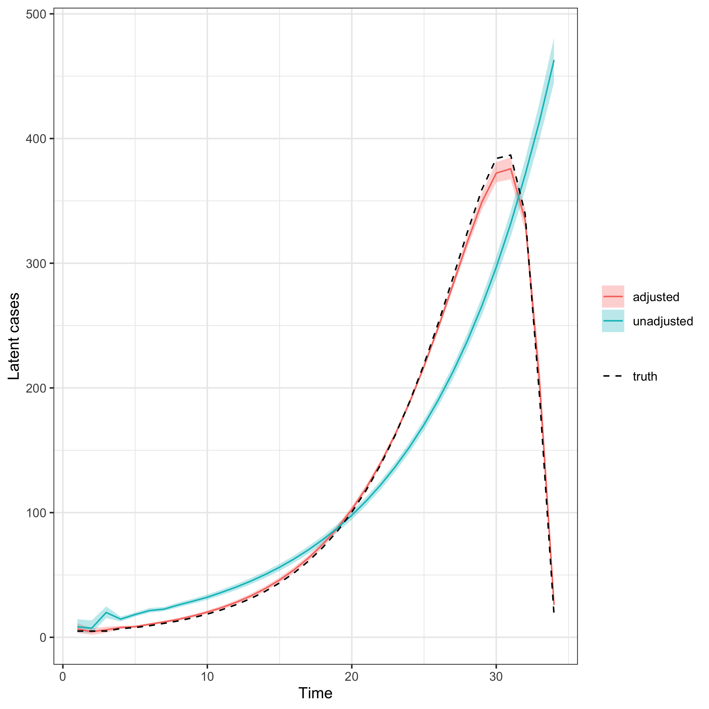

Posterior latent cases (90% credible interval) under each model against the simulated truth.

Fitting an uncertain population

When the initial susceptible population is unknown, it can be estimated by setting population_uncertain = TRUE. population then provides the median of a LogNormal prior with coefficient of variation population_cv.

Code

nowcast_uncertain <- epinowcast(
  pobs,
  expectation = enw_expectation(
    r = ~1, generation_time = gt, population = population,
    population_uncertain = TRUE, population_cv = 0.5, data = pobs
  ),
  obs = enw_obs(family = "poisson", data = pobs),
  fit = fit_opts
)

We plot the full posterior of the estimated population against the true value used to simulate the data. The posterior concentrates around the truth, showing the population is recovered from the depletion signal alone.

Code

pop_draws <- data.table(
  pop_est = as.numeric(
    posterior::as_draws_matrix(
      nowcast_uncertain$fit[[1]]$draws("expr_pop_est")
    )
  )
)

ggplot(pop_draws, aes(x = pop_est)) +
  geom_density(fill = "steelblue", alpha = 0.4) +
  geom_vline(
    aes(xintercept = population, linetype = "truth"), colour = "black"
  ) +
  scale_linetype_manual(values = c(truth = "dashed")) +
  labs(
    x = "Initial susceptible population", y = "Posterior density",
    linetype = NULL
  ) +
  theme_bw()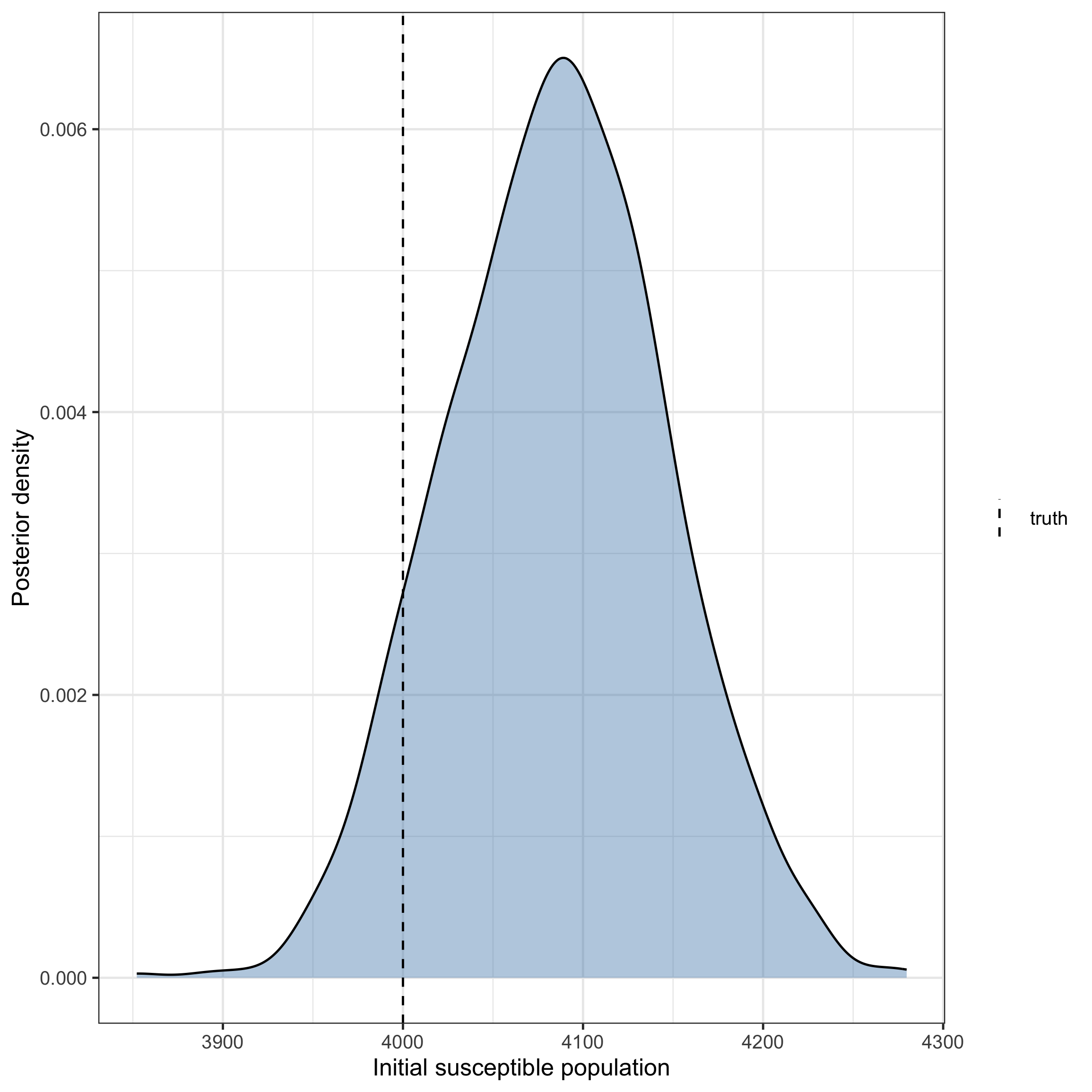

Posterior of the estimated initial susceptible population against the true value (dashed line).

Assumptions

The adjustment assumes a single well-mixed population per group with no waning of immunity and no births or deaths, so the susceptible pool is only ever depleted by modelled latent cases. It applies only to the renewal path (length(generation_time) > 1). The model vignette describes the adjustment and gives the references for the susceptible-depletion form it follows. See ?enw_expectation for the population, population_floor, population_uncertain, and population_cv arguments.